


-
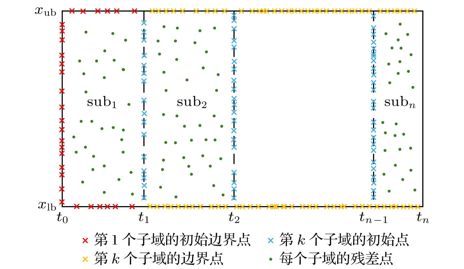
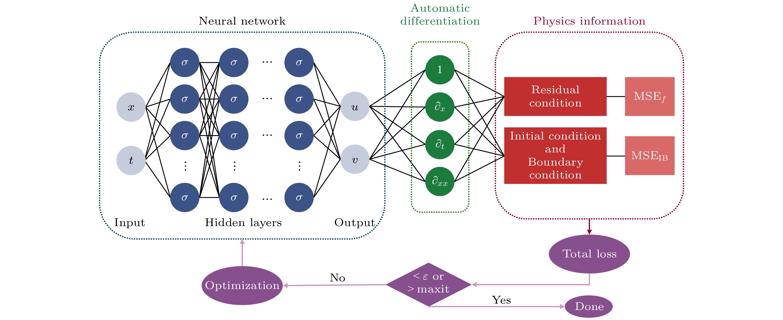
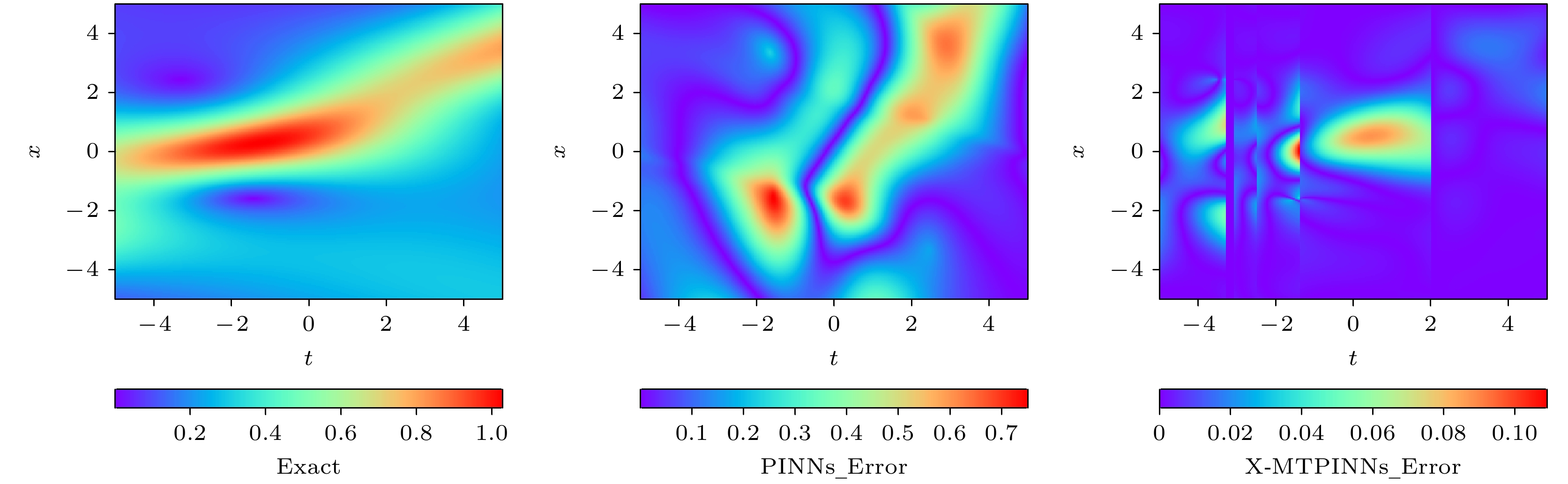
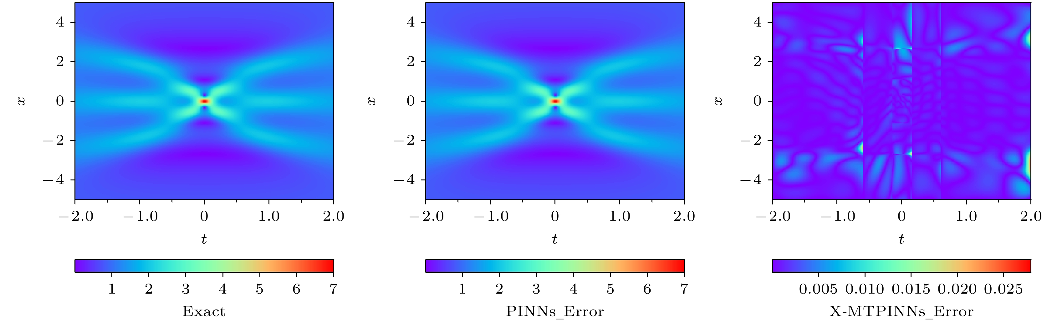
In recent years, physics-informed neural networks (PINNs) have provided effcient data-driven methods for solving forward and inverse problems of partial differential equations (PDEs). However, when addressing complex PDEs, PINNs face significant challenges in computational efficiency and accuracy. In this study, we propose the extended mixed-training physics-informed neural networks (X-MTPINNs) as illustrated in the following figure, which effectively enhance the ability to solve nonlinear wave problems by integrating the domain decomposition technique of extended physics-informed neural networks (X-PINNs) in a mixed-training physics-informed neural networks (MTPINNs) framework. Compared with the classical PINNs model, the new model exhibits dual advantages: The first advantage is that the mixed-training framework significantly improves convergence properties by optimizing the handling mechanism of initial and boundary conditions, achieving higher fitting accuracy for nonlinear wave solutions while reducing the computation time by approximately 40%. And the second advantage is that the domain decomposition technique from X-PINNs strengthens the ability of the model to represent complex dynamical behaviors. Numerical experiments based on the nonlinear Schrödinger equation (NLSE) demonstrate that X-MTPINNs excel perform well in solving two bright solitons, third-order rogue waves, and parameter inversion tasks, with prediction accuracy improved by one to two orders of magnitude over traditional PINN. For inverse problems, the X-MTPINNs algorithm accurately identifies unknown parameters in the NLSE under noise-free, 2%, and 5% noisy conditions, solving the complete failure problem of NSLE parameter identification in classical PINNs in the studied scenario, thus demonstrating strong robustness.
-
Keywords:
- physics-informed neural networks /
- nonlinear Schrödinger equation /
- extended mixed-training physics-informed neural networks /
- domain decomposition /
- parameter identification
[1] [2] [3] [4] [5] [6] [7] [8] [9] [10] [11] [12] [13] [14] [15] [16] [17] [18] [19] [20] [21] [22] [23] [24] [25] [26] [27] [28] [29] [30] [31] [32] [33] [34] [35] [36] -
亮双孤子 子域 隐藏
层数神经
元数L2误差 训练时间/s X-
MTPINNs[–5.00, –3.30] 4 50 4.52×10⁻² 2531.88 [–3.30, –2.50] 4 50 2.63×10⁻² 2459.23 [–2.50, –1.40] 4 50 3.03×10⁻² 2347.56 [–1.40, 2.00] 4 50 5.73×10⁻² 2489.87 [2.00, 5.00] 4 50 1.70×10⁻² 2489.87 Global [–5, 5] 4 50 3.38×10⁻² 2531.88 PINNs [–5, 5] 4 50 2.51×10⁻¹ 4176.69  DownLoad: CSV
三阶怪波 子域 隐藏
层数神经
元数L2误差 训练时间/s X-
MTPINNs[–2.00, –0.60] 4 50 1.25×10⁻³ 3065.07 [–0.60, –0.15] 4 50 1.22×10⁻³ 2228.26 [–0.15, 0.15] 4 50 3.89×10⁻³ 2018.29 [0.15, 0.60] 4 50 1.31×10⁻³ 2438.84 [0.60, 2.00] 4 50 1.84×10⁻³ 2339.57 Global [–2, 2] 4 50 2.25×10⁻³ 3065.07 PINNs [–2, 2] 4 50 4.94×10⁻¹ 5538.17
DownLoad: CSV
NPDEs 噪声 非线性演化方程 相对误差$ [\lambda_1, \lambda_2] $/% Correct — $ {\rm{i}}\hat{h}_t + 0.5\hat{h}_{xx} + |\hat{h}|^2\hat{h} = 0 $ $ [0, 0] $ [–2.00, –0.60] 0% $ \lambda_1 = 0.4999224, \lambda_2 = 0.9999491 $ $ [0.01553, 0.00509] $ 2% $ \lambda_1 = 0.5006779, \lambda_2 = 1.0010909 $ $ [0.13558, 0.10909] $ 5% $ \lambda_1 = 0.5017547, \lambda_2 = 1.0026274 $ $ [0.35094, 0.26274] $ [–0.60, –0.08] 0% $ \lambda_1 = 0.4995355, \lambda_2 = 0.9997470 $ $ [0.09289, 0.02530] $ 2% $ \lambda_1 = 0.4990919, \lambda_2 = 0.9979020 $ $ [0.18162, 0.20980] $ 5% $ \lambda_1 = 0.4983062, \lambda_2 = 0.9952767 $ $ [0.33876, 0.47233] $ [–0.08, 0.00] 0% $ \lambda_1 = 0.4907891, \lambda_2 = 0.9970491 $ $ [1.84218, 0.29509] $ 2% $ \lambda_1 = 0.4856022, \lambda_2 = 0.9931418 $ $ [2.87955, 0.68582] $ 5% $ \lambda_1 = 0.4838027, \lambda_2 = 0.9913622 $ $ [3.23946, 0.86378] $ [0.00, 0.08] 0% $ \lambda_1 = 0.4978686, \lambda_2 = 0.9941696 $ $ [0.42627, 0.58304] $ 2% $ \lambda_1 = 0.4953954, \lambda_2 = 0.9936743 $ $ [0.92092, 0.63257] $ 5% $ \lambda_1 = 0.4909737, \lambda_2 = 0.9887489 $ $ [1.80527, 1.12511] $ [0.08, 0.60] 0% $ \lambda_1 = 0.4999007, \lambda_2 = 0.9997627 $ $ [0.01987, 0.02373] $ 2% $ \lambda_1 = 0.4997132, \lambda_2 = 0.9992683 $ $ [0.05737, 0.07317] $ 5% $ \lambda_1 = 0.4974256, \lambda_2 = 0.9973150 $ $ [0.51489, 0.26850] $ [0.60, 2.00] 0% $ \lambda_1 = 0.5002598, \lambda_2 = 1.0001861 $ $ [0.05195, 0.01861] $ 2% $ \lambda_1 = 0.4997032, \lambda_2 = 0.9999705 $ $ [0.05936, 0.00295] $ 5% $ \lambda_1 = 0.4995049, \lambda_2 = 0.9998789 $ $ [0.09903, 0.01211] $ Global 0% $ \lambda_1 = 0.972926, \lambda_2 = 0.9987469 $ $ [0.54148, 0.12531] $ 2% $ \lambda_1 = 0.5035173, \lambda_2 = 0.9971460 $ $ [0.70345, 0.28540] $ 5% $ \lambda_1 = 4.9470665, \lambda_2 = 1.0050076 $ $ [1.05867, 0.50076] $
DownLoad: CSV
-
[1] [2] [3] [4] [5] [6] [7] [8] [9] [10] [11] [12] [13] [14] [15] [16] [17] [18] [19] [20] [21] [22] [23] [24] [25] [26] [27] [28] [29] [30] [31] [32] [33] [34] [35] [36]


 DownLoad:


Catalog
Metrics
- Abstract views: 621
- PDF Downloads: 14
- Cited By: 0